Fractional Delays

The beam steering process used with microphone arrays requires the ability to delay the signal from each microphone in order to align the incident wavefront of interest. When dealing with sampled data, it is highly likely that these delays will not equate to multiples of whole sample periods. This being the case, an implementation of a steerable beamformer will need to implement a fractional delay process.

Introduction

Delaying sampled data by a fraction of a sample period is a critical part of array beamforming. The image below shows two microphones with a plane wave approaching from an angle of 45 degrees. The wavefront will reach microphone A before microphone B. To virtually steer the array beam to point to the plane wave's direction of arrival, the signal received at microphone A must be delayed.

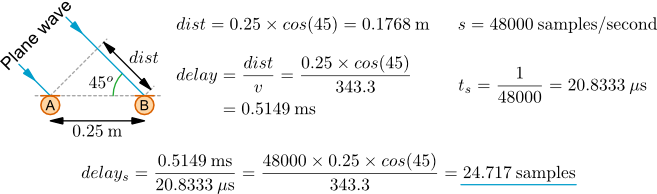
Given the microphone spacing of 0.25m and the plane wave arrival direction of 45°, the wavefront must travel a further 0.1768m to reach microphone B after reaching microphone A. If the speed of sound is taken as 343.3m/s this equates to 0.5149ms. Therefore, as shown in the image below, to align the two microphone signals, the signal from microphone A must be delayed by 0.5149ms.

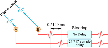
If the microphone signals are sampled at a rate of 48000 samples/second, then the delay of 0.5149ms is equivalent to a delay of 24.717 samples. The integer part of this delay is very simple to achieve with a basic buffer. However, the fractional part of 0.717 samples is more complicated and is the subject of this page.

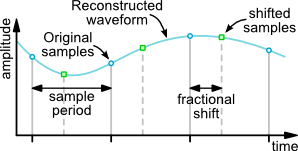
An approach to fractional delays is shown in the image below. The original waveform is reconstructed using the sampled data. The fractionally shifted samples are them created using by resampling. This is essentially the approach used in the two techniques described below.

Delay using a FIR filter

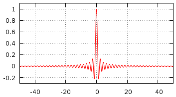
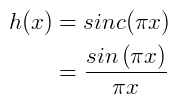
Based on the Nyquist-Shannon sampling theorem it is possible to recreate the original signal from sampled data by multiplying each sample by a scaled sinc function. The only condition is that the original waveform is bandlimited to have a maximum frequency component of less that half the sampling rate. So for a signal sampled at 48000 samples per second the maximum component frequency must be less than 24kHz.

Gnuplot commands for Sinc Function > h(x)=sin(pi*x)/(pi*x) > set xrange[-50:50] > set yrange[-0.3:1.1] > set samples 1000 > set grid > unset key > plot h(x)

Fractionally delayed reconstruction can be achieved by using a sinc function that is shifted by the fractional amount. This can then be implemented using a standard FIR filter structure. The plot below shows a sinc function with a fractional shift of 0.25. The weight values for a 11 tap FIR filter are also shown.

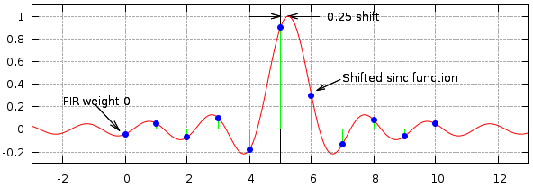
The sinc function is infinite along the x axis, however a FIR filter implementation requires a finite number of taps. Therefore, the final stage in implementing a fraction delay FIR filter is to window the shifted sinc function values. More information can be found on the FIR Filters by Windowing page.

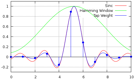
The plot below shows the how a Hamming window function is applied to the sinc function to calculate the tap weights for a 11 tap FIR delay filter. The table shows the calculated tap weight values.

Tap # Sinc Window Tap Weight 0 -0.042872 0.084682 -0.003631 1 0.052960 0.192355 0.010187 2 -0.069255 0.410403 -0.028423 3 0.100035 0.669597 0.066983 4 -0.180063 0.887645 -0.159832 5 0.900316 0.995318 0.896101 6 0.300105 0.958431 0.287630 7 -0.128617 0.788695 -0.101439 8 0.081847 0.540000 0.044197 9 -0.060021 0.291305 -0.017484 10 0.047385 0.121569 0.005761

The code below can be used to generate the tap weights for a given delay and filter length.

double delay = 0.25;               // Fractional delay amount
int filterLength = 11;             // Number of FIR filter taps (should be odd)
int centreTap = filterLength / 2;  // Position of centre FIR tap

for (int t=0 ; t<filterLength ; t++)
{
   // Calculated shifted x position
   double x = t - delay;

   // Calculate sinc function value
   double sinc = Math.sin(Math.PI * (x-centreTap)) / (Math.PI * (x-centreTap));

   // Calculate (Hamming) windowing function value
   double window = 0.54 - 0.46 * Math.cos(2.0 * Math.PI * (x+0.5) / filterLength);

   // Calculate tap weight
   double tapWeight = window * sinc;

   // Output information
   System.out.printf("%3d % f % f % f\n", t, sinc, window, tapWeight);
}

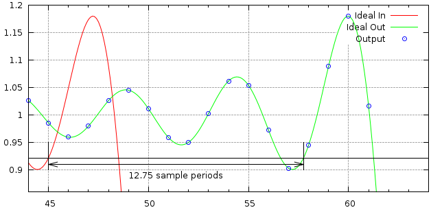
The plot below shows the delay generated by a 25 tap filter with a fractional delay of 0.75 samples using a Blackman windowing function. The 'Ideal In' curve shows the input signal, the 'Ideal Out' shows the same signal but delayed by 12.75 samples. The 'Output' points show the sample values generated at the output of the filter. It can be seen that these line up with the 'Ideal Out' curve. The delay is 12.75 samples rather than 0.75 samples due to the time it takes for the signal to propagate along the FIR filter taps.

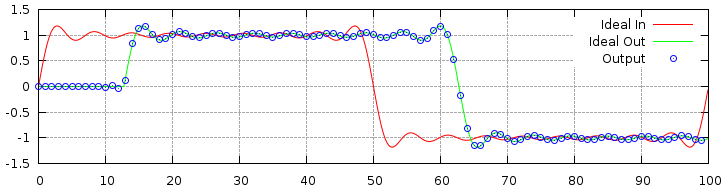
The following plot shows the delay between output and input more clearly.

The images below show the effect different windowing functions have on reconstruction accuracy.

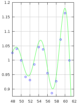
Rectangular Window

Hamming Window

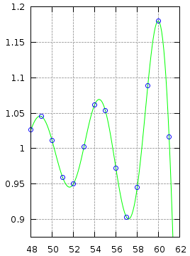
Blackman Window