Delay Calculation
A fundamental part of beamforming is calculating the differences in wave arrival time between array elements. The beamforming literature mainly uses two approaches; simple geometry, or vector dot product. This page describes using both methods how to calculate the time difference between a plane wave front arriving at an array element and an arbitrary reference point. A plane wave is normally assumed when the source is considered a long distance from the array.
Delay Calculation Using Basic Geometry
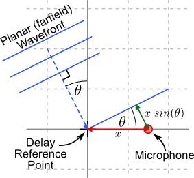
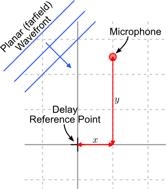
The left-hand image below shows a single microphone placed along the x axis. This reflects a single element position for a 1D array (right-hand image). In this setup, the angle of plane wave arrival is measured from the y axis; an angle of 0° is a broadside plane wave, an angle of ±90° is end-fire.
All delay measurements are taken with reference to a single point, in this case, the axis origin.
1D Delay Calculation |
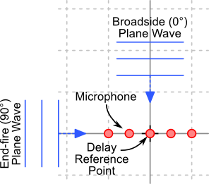
Linear array showing broadside and end-fire plane waves |
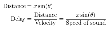
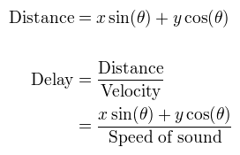
The wavefront time delay is calculated using the difference in distance a wave front must travel between the reference point and the element on interest. The time is then calculated by dividing this distance by the speed of sound.
The 2D case is shown below. The same basic approach is taken; calculate the difference in distance a wave front must travel between the origin and the element, then divide by the speed of sound. However, this time the distance calculation is for 2D.
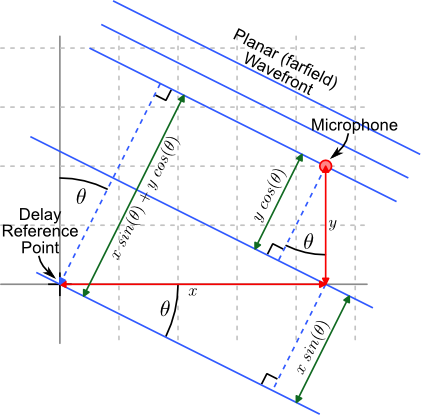
2D Delay Calculation |
|
Delay Calculation Using Vector Dot Product
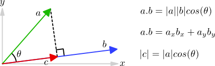
The vector dot product provides a simple approach of calculating wavefront delays. The image below shows three vectors. Vector c is the projection of vector a on to b. The length of vector c is known as the the scalar projection of a on to b. It is this projection that provides the method for calculating the wavefront delay.
Scalar Projection
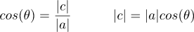
Using standard geometry of a right angle triangle, we can find the length of vector c, from the length of vector a and the angle between the two vectors.
Taking the dot product equation we can rearrange to find the length of vector c in terms of the dot-product of vectors a and b and the length of vector b.
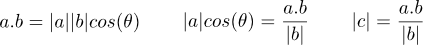
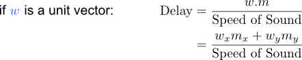
Finally, if we can ensure that vector b is a unit vector (has a length of 1), then the length of vector c is simply the dot-product of vectors a and b.

The images below show how the vector dot product can be applied to calculating the wavefront delay. The two vectors used are the element (microphone) position vector and the wavefront vector.
2D Microphone position |
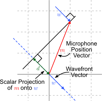
Dot Product Delay Calculation |
If the wavefront vector is a unit vector then the wavefront delay between the element and the origin can be calculated as follows.
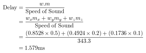
Example
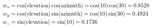
Here is an example of using the dot product to calculate the wave front delay for an array microphone in 3D space. An example microphone coordinates and wavefront source direction are given below. Please see the 3D coordinates systems page for a description of how these coordinates relate to each other.
|
|
First the wavefront direction is converted into a unit vector.
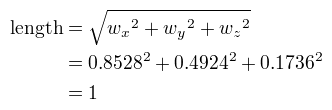
A quick check using Pythagoras' theorem, shows this is a unit vector.
Then the delay is calculated